Colorectal cancer incidence and mortality
Taavi Päll
2018-02-12
The aim of the vignette is to give some basic idea about the workflow when accessing Estonian Health Statistics and Health Research (TAI) datasets via boulder package.
Download list of available datasets
Data tables available on TAI database are listed in the data frame generated by get_all_tables() function. By default, datasets table is loaded from a local copy supplied with the package (local = TRUE). Set argument local = FALSE to download fresh list of tables from TAI.
Table columns Database and Node describe table address in the database tree. Database names are available only in Estonian.
- Name column contains table names and should be used when downloading data.
- Title columns contains table descriptions and in many cases also what are the values presented in the table (e.g. age-adjusted incidence per 100’000).
Updated and url contain date of the last update and data table url, respectively.
library(dplyr)
library(stringr)
library(tidyr)
library(ggplot2)
library(viridis)
library(boulder)
tabs <- get_all_tables(lang = "en")
tabs
#> # A tibble: 1,688 x 6
#>    Database    Node                         Name  Title    Updated  url
#>    <chr>       <chr>                        <chr> <chr>    <chr>    <chr>
#>  1 01Rahvastik Abortions                    RK01  Abortio… 2017-06… http:…
#>  2 01Rahvastik Abortions                    RK11  Abortio… 2017-11… http:…
#>  3 01Rahvastik Abortions                    RK20  Abortio… 2017-06… http:…
#>  4 01Rahvastik Abortions                    RK30  Abortio… 2017-06… http:…
#>  5 01Rahvastik Abortions                    RK40  Abortio… 2017-06… http:…
#>  6 01Rahvastik Abortions                    RK50  Use of … 2017-06… http:…
#>  7 01Rahvastik Abortions                    RK61  Legally… 2017-06… http:…
#>  8 01Rahvastik Abortions                    RK62  Abortio… 2017-06… http:…
#>  9 01Rahvastik Abortions                    RK63  Abortio… 2017-06… http:…
#> 10 01Rahvastik Births and breastfed infants SR01  Live bi… 2017-10… http:…
#> # ... with 1,678 more rows
Table info is stored in Title column. For better matching we convert Title column to lower case.
When looking for tables of interest it might be good idea to consult TAI database website, because, while database and node names, and table titles have nicely human readable descriptions, naming feels sometimes inconsistent and nonintuitive (at least to the author).
Cancer incidence
Cancer morbidity data is stored under Malignant neoplasms node.
tabs %>%
  mutate(descr = str_to_lower(Title)) %>%
  filter(str_detect(descr, "neoplasm")) %>%
  select(Name, Title, Node, Updated) %>%
knitr::kable()| Name | Title | Node | Updated |
|---|---|---|---|
| PK10 | New cases of malignant neoplasms by specified site, sex and age group | Malignant neoplasms | 2017-12-13T22:52:47 |
| PK20 | New cases of malignant neoplasms by specified site, sex and county | Malignant neoplasms | 2017-12-13T21:27:14 |
| PK30 | Age-specific incidence rate of malignant neoplasms per 100 000 inhabitants by site and sex | Malignant neoplasms | 2017-12-13T22:55:51 |
| PK40 | Incidence rate of malignant neoplasms per 100 000 inhabitants by specified site, sex and county | Malignant neoplasms | 2017-12-13T21:26:14 |
We are interested in table PK30: Age-specific incidence rate of malignant neoplasms per 100 000 inhabitants by site and sex.
pk30 <- pull_table("PK30", lang = "en")
pk30
#> # A tibble: 42,048 x 5
#>    Year  Site                              Sex   `Age group`  value
#>    <chr> <chr>                             <chr> <chr>        <dbl>
#>  1 2000  All malignant neoplasms (C00-C97) Men   0-4          18.5
#>  2 2000  All malignant neoplasms (C00-C97) Men   5-9          12.3
#>  3 2000  All malignant neoplasms (C00-C97) Men   10-14        11.1
#>  4 2000  All malignant neoplasms (C00-C97) Men   15-19         7.61
#>  5 2000  All malignant neoplasms (C00-C97) Men   20-24        25.8
#>  6 2000  All malignant neoplasms (C00-C97) Men   25-29        33.6
#>  7 2000  All malignant neoplasms (C00-C97) Men   30-34        36.3
#>  8 2000  All malignant neoplasms (C00-C97) Men   35-39        75.0
#>  9 2000  All malignant neoplasms (C00-C97) Men   40-44       143
#> 10 2000  All malignant neoplasms (C00-C97) Men   45-49       247
#> # ... with 42,038 more rows
Let’s see if we can find data for colon cancer incidence. Cancer anatomical site is stored under Site variable. Incidence values are available for 73 anatomical sites.
pk30 %>%
  select(Site) %>%
  distinct()
#> # A tibble: 73 x 1
#>    Site
#>    <chr>
#>  1 All malignant neoplasms (C00-C97)
#>  2 All malignant neoplasms except skin (other) (C00-C97, except C44)
#>  3 Lip, oral cavity and pharynx (C00-C14)
#>  4 ..Lip (C00)
#>  5 ..Tongue (C01-02)
#>  6 ..Gum, floor of mouth etc (C03-C06)
#>  7 ..Major salivary glands (C07-C08)
#>  8 ..Tonsil, oropharynx (C09-C10)
#>  9 ..Nasopharynx (C11)
#> 10 ..Piriform sinus, hypopharynx (C12-C13)
#> # ... with 63 more rows
After some digging, we can see that colon cancer is nested under Digestive organs (C15-C26): ..Colon (C18). Now we can pull out data for colon regular expression.
colo <- pk30 %>%
  mutate_at("Site", str_to_lower) %>%
  filter(str_detect(Site, "colon"))
colo
#> # A tibble: 576 x 5
#>    Year  Site          Sex   `Age group` value
#>    <chr> <chr>         <chr> <chr>       <dbl>
#>  1 2000  ..colon (c18) Men   0-4          0
#>  2 2000  ..colon (c18) Men   5-9          0
#>  3 2000  ..colon (c18) Men   10-14        0
#>  4 2000  ..colon (c18) Men   15-19        0
#>  5 2000  ..colon (c18) Men   20-24        0
#>  6 2000  ..colon (c18) Men   25-29        0
#>  7 2000  ..colon (c18) Men   30-34        2.13
#>  8 2000  ..colon (c18) Men   35-39        0
#>  9 2000  ..colon (c18) Men   40-44        6.04
#> 10 2000  ..colon (c18) Men   45-49       10.8
#> # ... with 566 more rows
We have incidence rates for different age groups for men and women from years 2000 to 2015. Let’s plot incidence (value) versus time (Year) to see if there are any changes in incidence rates during this time period. First we also need to convert Year from character to numeric and Age group to factor to keep its correct ordering.
colo %>%
  mutate(Year = as.numeric(Year),
         `Age group` = factor(`Age group`, levels = unique(colo$`Age group`)),
         Site = gsub("^[.]+([a-z])", "\\U\\1", Site, perl = TRUE)) %>%
  ggplot(aes(Year, value, group = `Age group`, color = `Age group`)) +
  geom_line() +
  facet_wrap(~ Sex) +
  scale_color_viridis(discrete = TRUE) +
  guides(color = guide_legend(ncol = 2)) +
  labs(title = "Incidence of colon (C18) cancer",
       y = "Age-specific incidence per 100 000")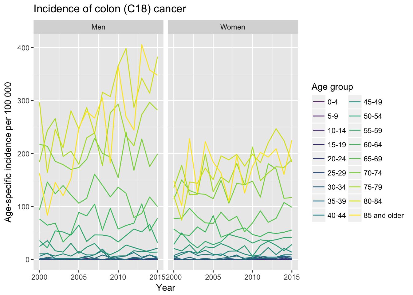
We can see that, as expected, cancer incidence is higher in older age groups (coloring) and colon cancer is generally higher in men. However, it is interesting that colon cancer incidence has been increasing in men during observed period.
Cancer mortality
Mortality data is stored under node Deaths.
tabs %>%
  mutate(Node = str_to_lower(Node)) %>%
  filter(str_detect(Node, "deaths"))
#> # A tibble: 15 x 6
#>    Database    Node   Name  Title                Updated   url
#>    <chr>       <chr>  <chr> <chr>                <chr>     <chr>
#>  1 01Rahvastik deaths SD21  Deaths by cause, se… 2018-01-… http://pxweb.t…
#>  2 01Rahvastik deaths SD22  Deaths per 100 000 … 2017-05-… http://pxweb.t…
#>  3 01Rahvastik deaths SD23  Standardised mortal… 2017-05-… http://pxweb.t…
#>  4 01Rahvastik deaths SD30  Deaths by sex, caus… 2017-05-… http://pxweb.t…
#>  5 01Rahvastik deaths SD31  15 prevalent causes… 2017-05-… http://pxweb.t…
#>  6 01Rahvastik deaths SD40  Deaths from disease… 2017-05-… http://pxweb.t…
#>  7 01Rahvastik deaths SD41  Direct drug-related… 2017-05-… http://pxweb.t…
#>  8 01Rahvastik deaths SD50  Infant deaths by se… 2017-05-… http://pxweb.t…
#>  9 01Rahvastik deaths SD501 Infant deaths by ca… 2017-05-… http://pxweb.t…
#> 10 01Rahvastik deaths SD51  Perinatal deaths by… 2017-05-… http://pxweb.t…
#> 11 01Rahvastik deaths SD52  Perinatal deaths an… 2017-06-… http://pxweb.t…
#> 12 01Rahvastik deaths SD53  Stillbirths by caus… 2017-05-… http://pxweb.t…
#> 13 01Rahvastik deaths SD60  Amenable deaths to … 2017-11-… http://pxweb.t…
#> 14 01Rahvastik deaths SD61  Preventable deaths … 2017-05-… http://pxweb.t…
#> 15 01Rahvastik deaths DR90  Autopsies            2017-05-… http://pxweb.t…
We are interested in table SD22 titled Deaths per 100 000 inhabitants by cause of death, sex and age group:
sd22 <- pull_table("SD22", lang = "en")
sd22
#> # A tibble: 99,960 x 5
#>    Year  `Cause of death`     Sex   `Age group`                  value
#>    <chr> <chr>                <chr> <chr>                        <dbl>
#>  1 1989  All causes (A00-Y89) Men   Crude mortality rate        1186
#>  2 1989  All causes (A00-Y89) Men   Standardised mortality rate   NA
#>  3 1989  All causes (A00-Y89) Men   0                           1775
#>  4 1989  All causes (A00-Y89) Men   1-4                          125
#>  5 1989  All causes (A00-Y89) Men   5-9                           74.1
#>  6 1989  All causes (A00-Y89) Men   10-14                         60.0
#>  7 1989  All causes (A00-Y89) Men   15-19                        165
#>  8 1989  All causes (A00-Y89) Men   20-24                        214
#>  9 1989  All causes (A00-Y89) Men   25-29                        223
#> 10 1989  All causes (A00-Y89) Men   30-34                        324
#> # ... with 99,950 more rows
It’s a relatively large table with 99960 rows. Let’s try to filter out colon and rectal cancer data using ICD codes. From incidence table we saw that this disease is placed under code C18.
mort <- sd22 %>%
  mutate(`Cause of death` = str_to_lower(`Cause of death`)) %>%
  filter(str_detect(`Cause of death`, "c18"))
mort
#> # A tibble: 2,352 x 5
#>    Year  `Cause of death`                     Sex   `Age group`      value
#>    <chr> <chr>                                <chr> <chr>            <dbl>
#>  1 1989  ....malignant neoplasm of colon and… Men   Crude mortality…  8.19
#>  2 1989  ....malignant neoplasm of colon and… Men   Standardised mo… NA
#>  3 1989  ....malignant neoplasm of colon and… Men   0                 0
#>  4 1989  ....malignant neoplasm of colon and… Men   1-4               0
#>  5 1989  ....malignant neoplasm of colon and… Men   5-9               0
#>  6 1989  ....malignant neoplasm of colon and… Men   10-14             0
#>  7 1989  ....malignant neoplasm of colon and… Men   15-19             0
#>  8 1989  ....malignant neoplasm of colon and… Men   20-24             0
#>  9 1989  ....malignant neoplasm of colon and… Men   25-29             0
#> 10 1989  ....malignant neoplasm of colon and… Men   30-34             0
#> # ... with 2,342 more rows
Let’s filter out data before year 2000 and keep only age groups data. Mortality is accounted separately for under 1 year old babies. Anyway, for comparison, we are mostly interested in >40 year old age groups, as cancer incidence is generally very low in younger people. Filter by Year and Age group:
colo_mort <- mort %>%
  filter(Year >= 2000,
         `Age group` %in% colo$`Age group`,
         !is.na(value))
colo_mort
#> # A tibble: 928 x 5
#>    Year  `Cause of death`                        Sex   `Age group` value
#>    <chr> <chr>                                   <chr> <chr>       <dbl>
#>  1 2001  ......malignant neoplasm of colon (c18) Men   5-9          0
#>  2 2001  ......malignant neoplasm of colon (c18) Men   10-14        0
#>  3 2001  ......malignant neoplasm of colon (c18) Men   15-19        0
#>  4 2001  ......malignant neoplasm of colon (c18) Men   20-24        0
#>  5 2001  ......malignant neoplasm of colon (c18) Men   25-29        0
#>  6 2001  ......malignant neoplasm of colon (c18) Men   30-34        0
#>  7 2001  ......malignant neoplasm of colon (c18) Men   35-39        0
#>  8 2001  ......malignant neoplasm of colon (c18) Men   40-44        2.02
#>  9 2001  ......malignant neoplasm of colon (c18) Men   45-49        6.47
#> 10 2001  ......malignant neoplasm of colon (c18) Men   50-54        9.49
#> # ... with 918 more rows
Now we can create similar plot as in case of incidence:
colo_mort %>%
  mutate(Year = as.numeric(Year),
         `Age group` = factor(`Age group`, levels = unique(colo_mort$`Age group`)),
         `Cause of death` = gsub("^[.]+([a-z])", "\\U\\1", `Cause of death`, perl = TRUE)) %>%
  ggplot(aes(Year, value, group = `Age group`, color = `Age group`)) +
  geom_line() +
  facet_wrap(~ Sex) +
  scale_color_viridis(discrete = TRUE) +
  guides(color = guide_legend(ncol = 2)) +
  labs(title = "Colon cancer (C18) mortality",
       y = "Deaths per 100 000")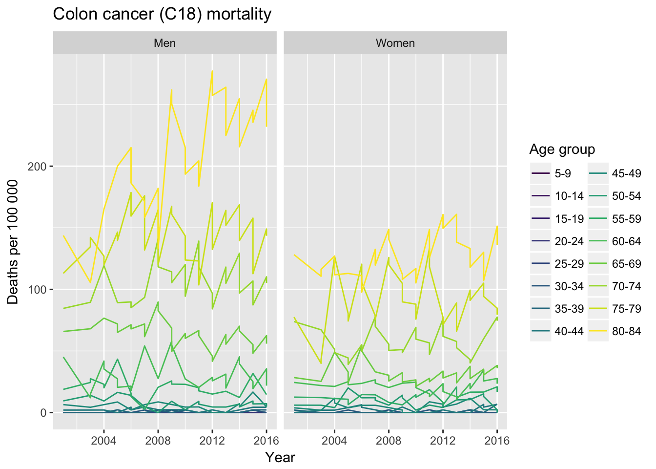
We can see that colon cancer deaths have shown considerable increase in 80-84 age group in men, whereas mortality among women has remained pretty much the same.
Incidence versus mortality
Cancer mortality can be considered as a proxy to treatment efficacy. Therefore, let’s put these two datasets side by side to get better visual at the gap between morbidity and mortality, and how deadly this disease really is in Estonia.
First, we need to merge incidence and mortality datasets:
c18 <- inner_join(
  colo %>% select(-Site) %>% rename(incidence = value),
  colo_mort %>% select(-`Cause of death`) %>% rename(mortality = value)
  ) %>%
  filter(incidence != 0)
c18
#> # A tibble: 580 x 5
#>    Year  Sex   `Age group` incidence mortality
#>    <chr> <chr> <chr>           <dbl>     <dbl>
#>  1 2001  Men   30-34            2.10      0
#>  2 2001  Men   35-39            4.19      0
#>  3 2001  Men   40-44           12.1       2.02
#>  4 2001  Men   45-49           10.8       6.47
#>  5 2001  Men   50-54           35.6       9.49
#>  6 2001  Men   55-59           22.0      18.8
#>  7 2001  Men   60-64           64.9      45.1
#>  8 2001  Men   65-69          146        65.8
#>  9 2001  Men   70-74          214        84.6
#> 10 2001  Men   75-79          243       113
#> # ... with 570 more rows
Now we can plot colon cancer incidence versus mortality, but first we want to gather incidence and mortality values into common column for easier plot setup:
c18 %>%
  mutate(Year = as.numeric(Year)) %>%
  gather(key, value, -c("Year", "Sex", "Age group")) %>%
  ggplot(aes(Year, value, color = key)) +
  geom_line() +
  facet_grid(Sex ~ `Age group`) +
  scale_color_viridis(discrete = TRUE, direction = -1) +
  theme(axis.text.x = element_text(angle = 90, vjust = 0.5, size = 6),
        legend.title = element_blank(),
        legend.position = "bottom") +
  labs(y = "Incidence vs. mortality per 100000")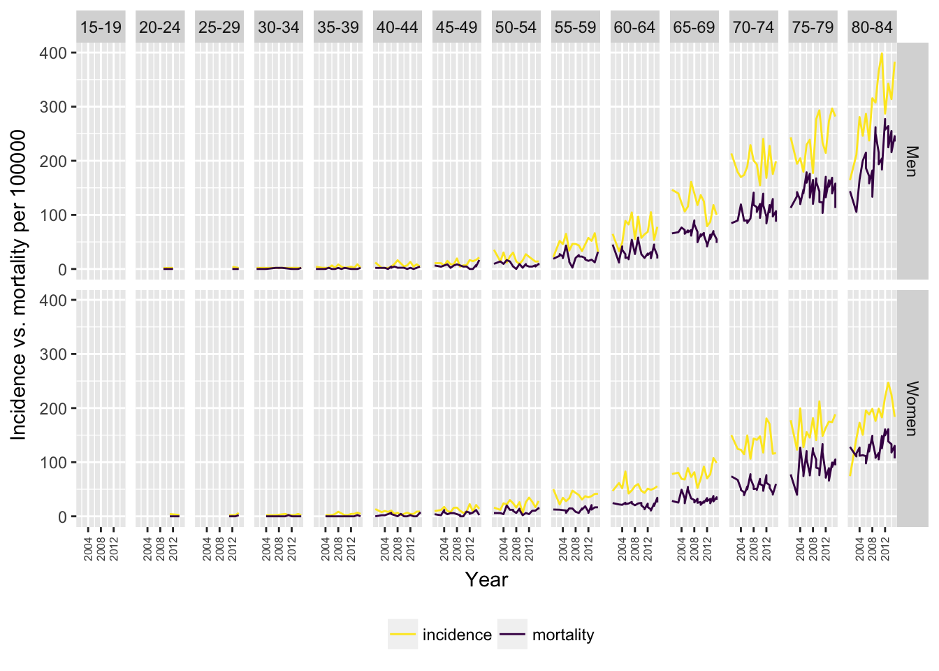
Summary
Ok, this is how working with TAI data basically looks like – find your table and download it, whereas it’s advisable to compare downloaded table to the one available on TAI webpage. Downloaded tables may need lot of cleaning (e.g. to get rid of summary data rows), pay attention to variable names which are nicely human readable but contain whitespace, may contain apostrophes.